![Learning better Point Cloud Representation using JEPA [Part 1]](/assets/images/projects/point-jepa/image.png)
You might have wondered how autonomous cars are able to “see” pedestrians, and cars at an unlit street at 2 am, they “see” them not as a picture but cluster of dots in 3D space, each one a precise coordinate bounced back by a LiDAR. No color. No texture. Just pure geometry, telling the car where any solid object is.
This cluster of dots in 3D Space is called Point Cloud. They are the outputs of LiDAR sensors on top of an autonomous car, and depth cameras. Each point cloud is a set of unordered (x, y, z) coordinates, representing a scene, or an object.
Because point clouds capture uncompromised 3D Geometry, they have become mission-critical anywhere that precise spatial measurement beats visual estimation.
- In Autonomous Vehicles, they allow them to track pedestrians, and obstacles in pitch-dark environment
- Used in Spatial Computing(AR/VR/MR) to constantly map your room.
Now, the question arises why can’t we just use the same CNNs we use to process Images? Because points clouds break one important principle CNNs are built on. An Image is a rigid grid: it always have the same neighbours, and convolution kernal can learn meaningful local patterns by sliding across this grid
Meanwhile, Point Clouds has no such grid. Point clouds are set of n unordered (x, y, z) coordinates, you can shuffle them n! times, and still get the same object. There is no concept of rigid grids in Point Clouds for the CNNs to exploit. This property is called Permutation Invariance.
The breakthrough came from an unlikely place: Images started to abandon the grid too. But in 2020, ViTs(Vision Transformers) made us realise that we don’t really any rigid local grinds to understand an Image, we can just chop them into patches, convert them into tokens, and feed these tokens into Transformers to figure out the relationship. This global understanding lead to creation of Point Cloud Transformers, and then powerful self-supervised models like Point-BERT, Point-MAE and Point-JEPA.
The first step in building any of these methods is converting a point cloud into tokens a Transformer can consume. Image models solved this by treating an image as worth 16×16 words. Is there a point-cloud equivalent? Let’s find out?
Converting Point Clouds into tokens
First, we need a dataset. We will be using ModelNet40 with 12, 311 shapes, 40 categories, and 2048 points per shape.
wget https://shapenet.cs.stanford.edu/media/modelnet40_ply_hdf5_2048.zip
unzip modelnet40_ply_hdf5_2048.zip
Now, we need to concatenate all the shapes from the .h5 files given in the dataset into two big numpy array of point clouds and labels, for both train and test, and then wrap them in a Dataset class which samples target no of points from each point clouds, and normalizes each point clouds.
class ModelNet40Dataset(Dataset):
    def __init__(self, data, labels, target_points=2048):
        self.data = data
        self.labels = labels
        self.target_points = target_points

    def __len__(self):
        return len(self.data)

    def __getitem__(self, idx):
        sample = self.data[idx]
        random_indices = np.random.choice(sample.shape[0], self.target_points, replace=False) #Sample random number of target points
        sample = sample[random_indices]
        sample = sample - sample.mean(axis=0)  #Center the point cloud
        sample = sample / np.linalg.norm(sample, axis=1).max()  #Normalize to unit sphere
        sample = sample.astype(np.float32)
        sample = torch.from_numpy(sample)
        label = self.labels[idx][0].astype(np.int64)
        label = torch.tensor(label)

        return sample, label
With the Dataset in place, and a standard DatsetLoader give us batches. Now, the real question arises, How can we convert Point Clouds into patches like Images?
Maybe, I can naively choose a point as a token, but this would lead to high computational cost later, since complexity of self-attention in transformer is quadratic.
Now, a simple and efficient method of converting point clouds in sub-clouds or patches is presented in Point-BERT, where they sample g center points from the point cloud p using Farthest Point Sampling, and then kNN algorithm is used to select the n nearest neighbour points from each center point.
The intution is simple: you want your center points to cover the whole shape as evenly as possible, so you want to space out the center points such that they overlap as little as possible. FPS does this greedily.
Farthest Point Sampling: Sampling Points Greedily
1. Pick a random starting point from the cloud and add it to our "selected" set.
2. For all remaining points, calculate their distance to the nearest selected point.
3. Find the point that has the maximum minimum distance to the selected set (i.e., the point furthest away from everything we've picked so far).
4. Add it to our selected set, and repeat until we have g center points.
def farthest_point_sampling(self, points_batches, num_samples):
        """
        Perform farthest point sampling on a set of points.

        Parameters:
        points_batches (torch.tensor): Input point cloud of shape (B, N, 3).
        num_samples (int): Number of points to sample.

        Returns:
        torch.tensor: Sampled points of shape (B, num_samples, 3).
        """

        B, N, _ = points_batches.shape #Batch size, N number of points, 3 coordinates

        sampled_indices = torch.zeros((B, num_samples), dtype=torch.int64).to(points_batches.device) #Batch size, num_samples

        distances = torch.full((B, N), float('inf')).to(points_batches.device) #Initialize distances to infinity for each point in the batch

        # Randomly select the first point
        sampled_indices[:, 0] = torch.randint(0, N, size=(B,)).to(points_batches.device) #[row_section, column_section] Assign a random index for each batch on the first column of sampled_indices

        for i in range(1, num_samples):
            # Update distances to the nearest sampled point
            last_sampled_points = points_batches[torch.arange(B)[:, None], sampled_indices[:, i - 1].reshape(-1, 1)] #Get the last sampled point for each batch
            dist_to_last_sampled = torch.cdist(points_batches, last_sampled_points)
            distances = torch.minimum(distances, dist_to_last_sampled.squeeze(-1))  # Update distances to the nearest sampled point

            # Select the farthest point
            sampled_indices[:, i] = torch.topk(distances, k=1, dim=1, largest=True).indices.squeeze(-1)

        return points_batches[torch.arange(B)[:, None], sampled_indices]
Once we have our evenly spaced out center points, each one can recruit its k closest point to form a local neighbourhood or sub-cloud.
def k_nearest_neighbors(self, points_batches, sampled_points_batches, k):
        """
        Find the k-nearest neighbors for each sampled point in a batch of point clouds.

        Parameters:
        points_batches (torch.tensor): Input point cloud of shape (B, N, 3).
        sampled_points_batches (torch.tensor): Sampled points of shape (B, M, 3).
        k (int): Number of nearest neighbors to find.

        Returns:
        torch.tensor: Indices of the k-nearest neighbors for each sampled point, shape (B, M, k).
        """

        B, N, _ = points_batches.shape
        _, M, _ = sampled_points_batches.shape

        # Compute pairwise distances between sampled points and all points
        distances = torch.cdist(sampled_points_batches, points_batches, p=2)  # Shape: (B, M, N)

        # Get the indices of the k-nearest neighbors
        knn_indices = torch.topk(distances, k=k, dim=-1, largest=False).indices  # Shape: (B, M, k)

        return knn_indices
Then, we combine these both to convert the point-clouds into sub-clouds.
 def tokenize(self, point_clouds):
        """
        Tokenize a batch of point clouds using farthest point sampling and k-nearest neighbors.

        Parameters:
        point_clouds (torch.Tensor): Input point cloud batch of shape (B, N, 3).

        Returns:
        tuple: Sampled points and their corresponding k-nearest neighbor indices.
        """

        sampled_points = self.farthest_point_sampling(point_clouds, self.num_samples)
        knn_indices = self.k_nearest_neighbors(point_clouds, sampled_points, self.k_neighbors)
        grouped_points = point_clouds[torch.arange(point_clouds.shape[0])[:, None, None], knn_indices]  # Shape: (B, M, k, 3)
        grouped_points = grouped_points - sampled_points.unsqueeze(2)  # Center the k-nearest neighbors around the sampled point

        return sampled_points, grouped_points
Grouped Points represent a (B, M, k, 3) dimensional vector, where B is batch-size, M is the patch, and k represents k nearest neighbours of the center points.
Right now, these grouped points is just geometry, and doesn’t mean anything to the transformer, and do not carry information about where in the object it is. So, we need to convert the Grouped points into token embeddings and the Sampled Points i.e the center points of each sub-cloud into positional embeddings.
Tokens represent the local shape geometry, and have no idea where they are present in the object, and to help with this we have positional embeddings, which tell the transformers where are these located in the 3D Point Cloud.
For this, we will employ a miniPointNet Encoder, which takes (B, M, K, 3) size tensor as input, and results in an (B, M, 128) ouput, where 128 is the token dimension.
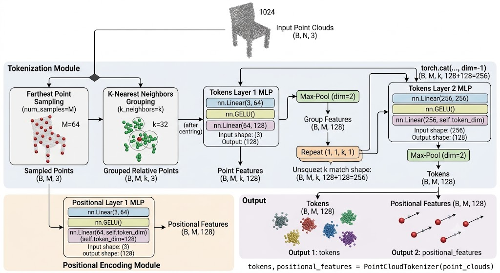
generated using AI
In the following architecture, we made some design choices:
- By centering the Grouped Points, we ensure translation invariance. This ensures that the local geometric features learned are identical regardless of where they are present in the 3D Point Cloud.
- By Max Pooling over the group, we ensure permutation invariance since max() yields the same output token, no matter how the points are arranged.
- By Concatenating the max pooled grouped features with point features, we enable it to understand the context of it’s k neighbours. Now, it does make the network Permutation Equivariant for now, but the second layer uses Max Pooling again to preserve the permutation invariance nature.
Using this architecture, we are able to get tokens and positional encoding of shape (B, M, 128) from unordered coordinates of a point cloud, which can now be fed into Transformer encoder.
What’s Next?
Let’s describe the real problem now: Since Label 3D Data is expensive, someone has to hand-annotate object categories, part segments, or scene semantics for every shape, we need self-supervised pre-training to learn general-purpose geometric representations from raw point clouds alone. We do this by training an encoder on a pretext task that needs no label at all, so it learns general-purpose geometric representations, and then later we fine tune on far lesser label data.
That raises the actual question this series wants to answer: what’s the best pretext task for pre-training a point cloud encoder?
We have two families which try to solve the problem differently:
- Reconstruction in Input Space: Methodology used by Point-BERT and Point-MAE. The idea is simple mask out a chunk of tokenized patches, and train the encoder to reconstruct the missing geometry. Point-BERT uses a pre-made catalog of missing pieces and geometry shapes to fill in the missing gap, while Point-MAE tries to draw the missing chunk, point by point.
- Prediction in latent Space: Methodology used by point2vec and Point-JEPA. The idea is to get a rough impression of the missing chunk, instead of reconstructing the missing geometry. Because, now the model is based on understanding rather than rendering, it learns better representation of the object’s shape and structure.
Now, the problem I am chasing is, does the Point-JEPA produce better, more efficient representations than Point-BERT and Point-MAE?
Supervised Baseline
But before moving to self-supervision, we need a supervised baseline. This is the accuracy that Point-JEPA has to beat. It’s the simplest thing that could work: feed the tokens straight into a plain transformer encoder, and train the whole thing end-to-end with the ModelNet40 labels using ordinary cross-entropy.
Let’s start simple and then progressively move to creating a powerful baseline.
class BaselineModel(nn.Module):
    def __init__(self, tokenizer):
        super(BaselineModel, self).__init__()
        self.tokenizer = tokenizer
        self.encoder_layer = nn.TransformerEncoderLayer(d_model=128, nhead=4, dim_feedforward=512, batch_first=True, activation='gelu')
        self.encoder = nn.TransformerEncoder(self.encoder_layer, num_layers=4)

        self.linear_head = nn.Linear(tokenizer.token_dim, 40)  # Assuming 40 classes for ModelNet40

    def forward(self, x):
        tokens, positional_embeddings = self.tokenizer(x)
        combined_tokens = tokens + positional_embeddings  # Combine tokens with positional embeddings
        x = self.encoder(combined_tokens)
        x = torch.mean(x, dim=1)  # Global average pooling over the sequence length
        x = self.linear_head(x)
        return x
Raw point clouds go in, the tokenizer produces patch tokens and their positional embeddings, the two get added together the way ViT combines patch and position embeddings, and a standard Transformer encoder attends over the whole sequence.
Early runs used a flat 3e-4 learning rate with AdamW’s default weight decay(0.01), then I noticed the training was noisy in the first few epochs, so I added a 2-epoch linear warmup into cosine annealing, which smoothed that out.
After I noticed that the training accuracy climped over 97% and my test accuracy was stuck at around 84-85%. I decided to use Data Augmentation. I added random gaussian noise to the point clouds, random scaling factor and random rotation around y axis. Honestly, it didn’t help much for some reason, my test accuracy barely climbed. So, I decided to change the architecture.
class BaselineModel(nn.Module):
    def __init__(self, tokenizer):
        super(BaselineModel, self).__init__()
        self.tokenizer = tokenizer
        self.encoder_layer = nn.TransformerEncoderLayer(d_model=128, nhead=4, dim_feedforward=512, batch_first=True, activation='gelu')
        self.encoder = nn.TransformerEncoder(self.encoder_layer, num_layers=2)
        self.cls_token = nn.Parameter(torch.randn(1, 1, tokenizer.token_dim) * 0.02)

        self.head_count = nn.Dropout(0.3)

        self.linear_head = nn.Linear(tokenizer.token_dim * 2, 40)  # Assuming 40 classes for ModelNet40

    def forward(self, x):
        tokens, positional_embeddings = self.tokenizer(x)
        combined_tokens = tokens + positional_embeddings  # Combine tokens with positional embeddings
        combined_tokens_shaped = combined_tokens.shape[0]
        cls = self.cls_token.expand(combined_tokens_shaped, -1, -1)  # Expand cls token to match batch size
        combined_tokens = torch.cat((cls, combined_tokens), dim=1)  # Concatenate cls token with the combined tokens
        x = self.encoder(combined_tokens)
        cls_token = x[:, 0, :]  # Extract the cls token representation
        max_pooled, _ = torch.max(x[:, 1:, :], dim=1)  # Max pooling over the token dimension (excluding cls token)
        x = torch.cat((cls_token, max_pooled), dim=-1)  # Concatenate cls token representation with max pooled representation
        x = self.head_count(x)
        x = self.linear_head(x)
        return x
Since, model was overfitting, I decided to reduce the number of layers of the Encoder to restrict model capacity to force it to generalize the data instead of memorizing the data.
Another, interesting thing, CLS Token, borrowed from ViTs and BERT, this token act as an empty backet which travel through the attention layers alongside your geometric tokens, and serves as the summary vector of my patch, but adding it wasn’t enough since in shallow transformers, CLS token doesn’t always have enough layer-depth to completely capture fine-grained structural edges. Hence, I used a max pooling operation to preserve the distinct geometries across all the patches.
So, after more than 20 iterations over different lr, dropouts, and design choices. Here, we are:
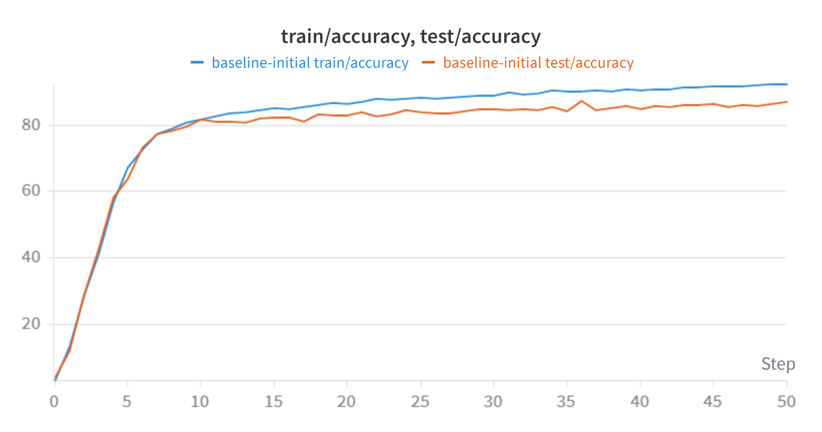
Training and Test Accuracy per Epoch
After around 40 epochs, the model converged with training accuracy 90.35% and test accuracy 87%,
Let’s see how well the model performs using various tests:
The very first test, I will perform is, checking the confusion matrix:
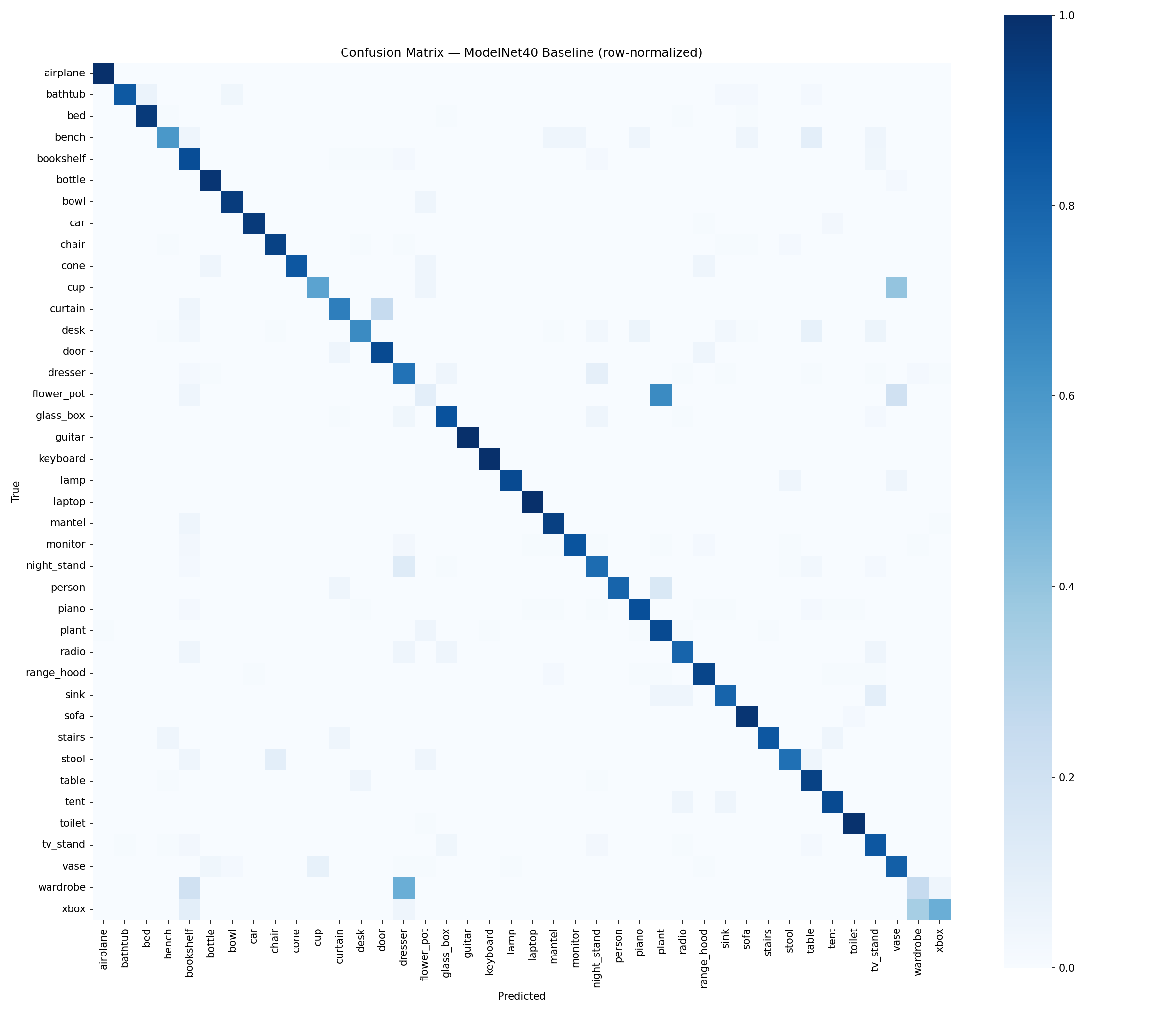
Confusion Matrix on 40 categories.
It simply tells us how many times it got it right, and how many times it got it wrong. The boxes on the diagonal simply mean, that the model made right prediction here whilst others are wrong predictions.
Now, if we see the plot clearly, model is confused in two cases: a. Flower Pot/Vase/Plant : genuinely ambigious categories b. Wardrobe/Dresser/Bookshelf/Night_stand: categories with similar bounding geometry
Top 10 confused pairs (true → predicted, count):
- flower_pot → plant : 13
- night_stand → dresser : 11
- wardrobe → dresser : 10
- vase → cup : 8
- dresser → night_stand : 8
- cup → vase : 8
- xbox → wardrobe : 7
- desk → table : 7
- table → desk : 5
- plant → flower_pot : 5
Errors aren’t uniformly distributed across categories, they concentrate almost entirely on pairs that are either semantically overlapping, or share similar coarse geometry despite different function. This suggests the baseline is learning real shape structure rather than memorizing noise.
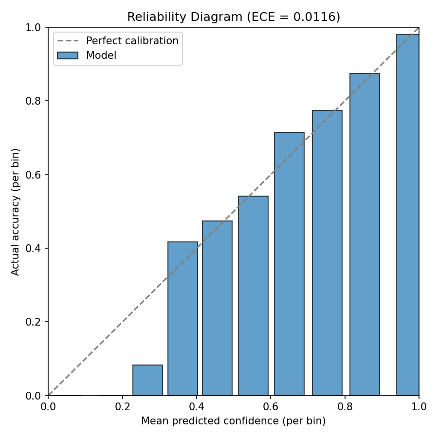
Reliability diagram
Now, this reliability diagram shows us the if the model is predicting a class with 80% confidence, it is right 80% of the times, and if it was correct only 60% of the times, then the model is said to be over-confident.
| Bin (x-position ≈) | Bar height (actual accuracy) | Above or below line? |
|---|---|---|
| ~0.25 | ~0.08 | Below — model is overconfident here |
| ~0.35 | ~0.42 | Above — underconfident |
| ~0.43 | ~0.47 | Above — underconfident |
| ~0.53 | ~0.54 | Roughly on the line |
| ~0.62 | ~0.72 | Above — underconfident |
| ~0.72 | ~0.77 | Above — underconfident |
| ~0.82 | ~0.87 | Above — underconfident |
| ~0.95 | ~0.98 | Above (slightly) — nearly perfect |
The reliability diagram shows real gaps in the mid-confidence bins, but the low overall ECE (0.0116) is mostly explained by the fact that most predictions live in the high-confidence bins, where the model is nearly exactly calibrated.
What’s next?
In Part-2, we will pre-train the same tokenizer + transformer architecture with Point-JEPA’s self-supervised objective i.e no labels, just predicting the latent representation of maskes patches from context.